#library(RWordPress)
#library(XMLRPC)
library(RISmed)
library(tm)
library(wordcloud2)
library(RColorBrewer)
library(topicmodels)
wordcloud
この記事はStanアドカレ14日目のエントリーです。今回のテーマはwordcloud、LDAです。wordcloudはしたの図にあるように、文章中で出現頻度が高い単語を複数選び出し、その頻度に応じた大きさで図示する手法で、単語の出現頻度が視覚的に理解できて便利。なによりイケてる。RではテキストデータをCorpusやdataframeとして整えてあげれば(ここがくっそ面倒)、wordcloudやwordcloud2といったパッケージで簡単にwordcloudを作成できます。特にwordcloud2は、以下のようにカッコ良い感じに仕上げてくれます。wordcloud2では文字の上に単語をのせるlettorcloudも可能です。
letterCloud(subset(term.f,freq>=3), word = "Stan",
            fontFamily = "Helvetica",
            wordSize=2, backgroundColor="white")
pubmedから論文情報をRStudioにぶち込む
上記のワードクラウドは、Pubmedでbayesianという検索用語でヒットした48本の英語論文のアブストラクトのテキストデータの単語の出現頻度に応じてプロットしたものです。以下のようにRISmedを用いると、Pubmedから簡単に論文情報を入手できます。
res <- EUtilsSummary("bayesian",#検索用語
                     type = "esearch",
                     db = "pubmed",
                     datetype = "pdat",
                     mindate = 2014, #検索開始年
                     maxdate = 2017, #検索終了年
                     retmax = 50 #最高何件記録するか
                     )
EUtilsSummary関数は検索演算子を発生させる関数になります。検索用語や検索開始、終了年を指定します。EUtilsGet関数で、論文情報を抜き出し格納します。そこからTitle情報を抜き出したいときはArticleTitle関数、アブストテキスト情報を抜き出したいときはAbstractText関数が使えます。
  records = EUtilsGet(res) #論文情報の抜き出し
  pubmed_data <- data.frame(Title = ArticleTitle(records),
                            Abstract = AbstractText(records))
こんな感じで論文のアブストテキストデータが抽出されました。今回は、この論文一つ一つのアブストテキストデータに対してトピックモデルの代表格であるLDAを適用し、それぞれの論文を潜在的なトピックにわりふって、トピックのまとまりごとにwordcloudを作ってやろう。というのが解析の目的になります。
  #データを確認
  library(knitr)
kable(head(pubmed_data,10))| Title | Abstract |
|---|---|
| Toxicogenetics of lopinavir/ritonavir in HIV-infected European patients. | AIMS: We present a genetic association study in 106 European HIV-infected individuals aimed at identifying and confirming polymorphisms that have a significant influence on toxicity derived from treatment with lopinavir/ritonavir (LPV/r).RESULTS: Suggestive relationships have been established between lipid plasma levels and total bilirubin and SNPs in CETP, MCP1, ABCC2, LEP and SLCO1B3 genes and between diarrhea and SNPs in IL6 gene.CONCLUSION: Replication analysis should confirm the novel results obtained in this study prior to its application in the clinical practice to achieve a safer LPV/r-based combined antiretroviral therapy. |
| Damage control laparotomy trial: design, rationale and implementation of a randomized controlled trial. | Damage control laparotomy (DCL) is an abbreviated operation intended to prevent the development of hypothermia, acidosis, and coagulopathy in seriously injured patients. The indications for DCL have since been broadened with no high-quality data to guide treatment. For patients with an indication for DCL, we aim to determine the effect of definitive laparotomy on patient morbidity.: Damage control laparotomy (DCL) is an abbreviated operation intended to prevent the development of hypothermia, acidosis, and coagulopathy in seriously injured patients. The indications for DCL have since been broadened with no high-quality data to guide treatment. For patients with an indication for DCL, we aim to determine the effect of definitive laparotomy on patient morbidity.This is a pragmatic, parallel-group, randomized controlled pilot trial. Emergent laparotomy is defined as admission directly to the operating room from the emergency department within 90 min of arrival. DCL indications excluded from the study include packing of the liver or retroperitoneum, abdominal compartment syndrome prophylaxis, to expedite interventional radiology for hemorrhage control, and the need for ongoing transfusions and/or continuous vasopressor support. When a surgeon determines a DCL is indicated, the patient will be screened for inclusion and exclusion criteria. Patients with any indication for DCL that is not excluded are eligible for randomization. Patients will be randomized intraoperatively to DCL (control) or definitive fascial closure of the laparotomy (intervention). The primary outcome will be major abdominal complication or death within 30 days. Major abdominal complication is a composite outcome including fascial dehiscence, organ/space surgical site infection, enteric suture line failure, and unplanned reopening of the abdomen. Outcomes will be compared using both frequentist and Bayesian statistics.: This is a pragmatic, parallel-group, randomized controlled pilot trial. Emergent laparotomy is defined as admission directly to the operating room from the emergency department within 90 min of arrival. DCL indications excluded from the study include packing of the liver or retroperitoneum, abdominal compartment syndrome prophylaxis, to expedite interventional radiology for hemorrhage control, and the need for ongoing transfusions and/or continuous vasopressor support. When a surgeon determines a DCL is indicated, the patient will be screened for inclusion and exclusion criteria. Patients with any indication for DCL that is not excluded are eligible for randomization. Patients will be randomized intraoperatively to DCL (control) or definitive fascial closure of the laparotomy (intervention). The primary outcome will be major abdominal complication or death within 30 days. Major abdominal complication is a composite outcome including fascial dehiscence, organ/space surgical site infection, enteric suture line failure, and unplanned reopening of the abdomen. Outcomes will be compared using both frequentist and Bayesian statistics.In patients with an indication for DCL, this trial will determine the effect of definitive laparotomy on major abdominal complications and death and will inform clinicians on the risks and benefits of this procedure. Regardless of the study outcome, the results will improve the quality of care provided to injured patients.: In patients with an indication for DCL, this trial will determine the effect of definitive laparotomy on major abdominal complications and death and will inform clinicians on the risks and benefits of this procedure. Regardless of the study outcome, the results will improve the quality of care provided to injured patients.NCT02706041.: NCT02706041. |
| Locally Adaptive Smoothing with Markov Random Fields and Shrinkage Priors. | |
| Bayesian regression model for recurrent event data with event-varying covariate effects and event effect. | In the course of hypertension, cardiovascular disease events (e.g., stroke, heart failure) occur frequently and recurrently. The scientific interest in such study may lie in the estimation of treatment effect while accounting for the correlation among event times. The correlation among recurrent event times come from two sources: subject-specific heterogeneity (e.g., varied lifestyles, genetic variations, and other unmeasurable effects) and event dependence (i.e., event incidences may change the risk of future recurrent events). Moreover, event incidences may change the disease progression so that there may exist event-varying covariate effects (the covariate effects may change after each event) and event effect (the effect of prior events on the future events). In this article, we propose a Bayesian regression model that not only accommodates correlation among recurrent events from both sources, but also explicitly characterizes the event-varying covariate effects and event effect. This model is especially useful in quantifying how the incidences of events change the effects of covariates and risk of future events. We compare the proposed model with several commonly used recurrent event models and apply our model to the motivating lipid-lowering trial (LLT) component of the Antihypertensive and Lipid-Lowering Treatment to Prevent Heart Attack Trial (ALLHAT) (ALLHAT-LLT). |
| A Bayesian spatio-temporal framework to identify outbreaks and examine environmental and social risk factors for infectious diseases monitored by routine surveillance. | |
| A Unified Analysis of Structured Sonar-terrain Data using Bayesian Functional Mixed Models. | Sonar emits pulses of sound and uses the reflected echoes to gain information about target objects. It offers a low cost, complementary sensing modality for small robotic platforms. While existing analytical approaches often assume independence across echoes, real sonar data can have more complicated structures due to device setup or experimental design. In this paper, we consider sonar echo data collected from multiple terrain substrates with a dual-channel sonar head. Our goals are to identify the differential sonar responses to terrains and study the effectiveness of this dual-channel design in discriminating targets. We describe a unified analytical framework that achieves these goals rigorously, simultaneously, and automatically. The analysis was done by treating the echo envelope signals as functional responses and the terrain/channel information as covariates in a functional regression setting. We adopt functional mixed models that facilitate the estimation of terrain and channel effects while capturing the complex hierarchical structure in data. This unified analytical framework incorporates both Gaussian models and robust models. We fit the models using a full Bayesian approach, which enables us to perform multiple inferential tasks under the same modeling framework, including selecting models, estimating the effects of interest, identifying significant local regions, discriminating terrain types, and describing the discriminatory power of local regions. Our analysis of the sonar-terrain data identifies time regions that reflect differential sonar responses to terrains. The discriminant analysis suggests that a multi- or dual-channel design achieves target identification performance comparable with or better than a single-channel design. |
| Mitochondrial-DNA Phylogenetic Information and the Reconstruction of Human Population History: The South American Case. | Mitochondrial DNA (mtDNA) sequences are becoming increasingly important in the study of human population history. Here, we explore the differences in the amount of information of different mtDNA regions and their utility for the reconstruction of South American population history. We analyzed six data sets comprising 259 mtDNA sequences from South America: Complete mtDNA, Coding, Control, hypervariable region I (HVRI), Control plus cytochrome b (cytb), and cytb plus 12S plus 16S. The amount of information in each data set was estimated employing several site-by-site and haplotype-based statistics, distances among sequences, neighbor-joining trees, distances among the estimated trees, Bayesian skyline plots, and phylogenetic informativeness profiles. The different mtDNA data sets have different amounts of information to reconstruct demographic events and phylogenetic trees with confidence. Whereas HVRI is not suitable for phylogenetic reconstruction of ancient clades, this region, as well as the Control data set, displays information for the demographic reconstruction during the Holocene period, probably because of the high rate of mutation of these regions. As expected, the Complete mtDNA and Coding data sets, displaying slower rates of mutation, present suitable information to estimate the founding subhaplogroups that populated South America and for the reconstruction of ancient demographic events. Our results point out the importance of evaluating the utility of different DNA regions to respond to different questions and problems in the human population studies, mainly considering the time scale of the phenomenon and the informativeness of the molecular region in a particular geographical area. |
| Estimating virus occurrence using Bayesian modeling in multiple drinking water systems of the United States. | Drinking water treatment plants rely on purification of contaminated source waters to provide communities with potable water. One group of possible contaminants are enteric viruses. Measurement of viral quantities in environmental water systems are often performed using polymerase chain reaction (PCR) or quantitative PCR (qPCR). However, true values may be underestimated due to challenges involved in a multi-step viral concentration process and due to PCR inhibition. In this study, water samples were concentrated from 25 drinking water treatment plants (DWTPs) across the US to study the occurrence of enteric viruses in source water and removal after treatment. The five different types of viruses studied were adenovirus, norovirus GI, norovirus GII, enterovirus, and polyomavirus. Quantitative PCR was performed on all samples to determine presence or absence of these viruses in each sample. Ten DWTPs showed presence of one or more viruses in source water, with four DWTPs having treated drinking water testing positive. Furthermore, PCR inhibition was assessed for each sample using an exogenous amplification control, which indicated that all of the DWTP samples, including source and treated water samples, had some level of inhibition, confirming that inhibition plays an important role in PCR-based assessments of environmental samples. PCR inhibition measurements, viral recovery, and other assessments were incorporated into a Bayesian model to more accurately determine viral load in both source and treated water. Results of the Bayesian model indicated that viruses are present in source water and treated water. By using a Bayesian framework that incorporates inhibition, as well as many other parameters that affect viral detection, this study offers an approach for more accurately estimating the occurrence of viral pathogens in environmental waters. |
| Vitrfication and Slow Freezing for Cryopreservation of Germinal Vesicle-Stage Human Oocytes: A Bayesian Meta-Analysis. | BACKGROUND: T he most commonly used methods for the cryopreservation of oocytes and embryos are vitrification and slow freezing.OBJECTIVE: The aim of this study was to to investigate whether there are differences in survival, in vitro maturation (IVM), and fertilization rates between cryopreserved immature oocytes, especially germinal vesicle (GV)-stage human oocytes, following vitrification and slow freezing.MATERIALS AND METHODS: A literature search was performed using the MEDLINE, Cochrane Central Register of Controlled Trials, and Embase databases. A total of three studies were included in the Bayesian meta-analysis.RESULTS: There was no difference in survival rates between vitrification and slow freezing. Additionally, there was no difference in IVM rates and fertilization rates between vitrification and slow freezing.CONCLUSION: The superiority of vitrification over slow freezing for cryopreservation of GV-stage human oocytes remains unclear. Additional studies on cytoarchitecture and modification of the cryopreservation protocol are essential to achieve strong conclusions. |
| Using the EM algorithm for Bayesian variable selection in logistic regression models with related covariates. | We develop a Bayesian variable selection method for logistic regression models that can simultaneously accommodate qualitative covariates and interaction terms under various heredity constraints. We use expectation-maximization variable selection (EMVS) with a deterministic annealing variant as the platform for our method, due to its proven flexibility and efficiency. We propose a variance adjustment of the priors for the coefficients of qualitative covariates, which controls false-positive rates, and a flexible parameterization for interaction terms, which accommodates user-specified heredity constraints. This method can handle all pairwise interaction terms as well as a subset of specific interactions. Using simulation, we show that this method selects associated covariates better than the grouped LASSO and the LASSO with heredity constraints in various exploratory research scenarios encountered in epidemiological studies. We apply our method to identify genetic and non-genetic risk factors associated with smoking experimentation in a cohort of Mexican-heritage adolescents. |
以下では、LDAを実施するためにテキストデータを整え、扱いやすくするためにCorpusデータに流していきます。論文の検索や下処理はもっともっと丁寧にやる必要がありますが、今回は飛ばします。
#Corpusで処理
pubmed_data$Abstract <- as.character(pubmed_data$Abstract)
docs <- Corpus(VectorSource(pubmed_data$Abstract))

docs <-tm_map(docs,content_transformer(tolower))
toSpace <- content_transformer(function(x, pattern) { return (gsub(pattern, " ", x))})
docs <- tm_map(docs, toSpace, "-")
docs <- tm_map(docs, toSpace, "’")
docs <- tm_map(docs, toSpace, "‘")
docs <- tm_map(docs, toSpace, "•")
docs <- tm_map(docs, toSpace, "”")

docs <- tm_map(docs, removePunctuation)
#Strip digits
docs <- tm_map(docs, removeNumbers)
#remove stopwords
docs <- tm_map(docs, removeWords, stopwords("english"))
#remove whitespace
docs <- tm_map(docs, stripWhitespace)
#Stem document
docs <- tm_map(docs,stemDocument)
#define and eliminate all custom stopwords
stops<-c("can", "say","one","way","use",
  "also","howev","tell","will",
  "much","need","take","tend","even",
  "like","particular","rather","said",
  "get","well","make","ask","come","end",
  "first","two","help","often","may",
  "might","see","someth","thing","point",
  "post","look","right","now","think","‘ve ",
  "‘re ","anoth","put","set","new","good",
  "want","sure","kind","larg","yes,","day","etc",
  "quit","sinc","attempt","lack","seen","awar",
  "littl","ever","moreov","though","found","abl",
  "enough","far","earli","away","achiev","draw",
  "last","never","brief","bit","entir","brief",
  "great","lot", "background", "aim", "method", "result", "conclusion",
  "show")

myStopwords <- stops

docs <- tm_map(docs, removeWords, myStopwords)
#inspect a document as a check
#delete.empty.docment
dtm <- DocumentTermMatrix(docs)
rowTotals <- apply(dtm , 1, sum) #Find the sum of words in each Document
empty.rows <- dtm[rowTotals == 0, ]$dimnames[1][[1]]
docs.new <- docs[-as.numeric(empty.rows)]
stanでLDA
さて、データが整ったので、LDAを実施しします。LDAで知りたいパラメタは2つ。一つは、どの文章がどのトピックに属する確率が高いかという、トピック分布(今回はtheta)。もう一つは、あるトピックはどのような用語が生起する確率が高いのかという、単語分布 (今回はphi)。 LDAをstanで書くと以下のようになります。コードは、こちらのブログを参考、というか丸パクリです。アヒル本にも、超わかりやすい解説あります。
data {
  int<lower=2> K;                    # num topics
  int<lower=2> V;                    # num words
  int<lower=1> M;                    # num docs
  int<lower=1> N;                    # total word instances
  int<lower=1,upper=V> W[N];         # word n
  int<lower=1> Freq[N];              # frequency of word n
  int<lower=1,upper=N> Offset[M,2];  # range of word index per doc
  vector<lower=0>[K] Alpha;          # topic prior
  vector<lower=0>[V] Beta;           # word prior
}
parameters {
  simplex[K] theta[M];   # topic dist for doc m
  simplex[V] phi[K];     # word dist for topic k
}
model {
  # prior
  for (m in 1:M)
    theta[m] ~ dirichlet(Alpha);
  for (k in 1:K)
    phi[k] ~ dirichlet(Beta);

  # likelihood
  for (m in 1:M) {
    for (n in Offset[m,1]:Offset[m,2]) {
      real gamma[K];
      for (k in 1:K)
        gamma[k] = log(theta[m,k]) + log(phi[k,W[n]]);
      increment_log_prob(Freq[n] * log_sum_exp(gamma));
    }
  }
}なお、今回は、複数のトピック数をためして見ましたがトピック数2以外がうまく分かれませんでした。HDPなど、トピック数の推定法、また時間があれば取り組んでみたいです。とりあえず、上記のコードをldatest.stanで保存し、以下のコードでキックして、(´д`)ハァハァします。
K=2 # トピック数
V=dtm.new$ncol # 単語数
M=dtm.new$nrow # 論文数
N=length(dtm.new$j) #総単語数
W<-dtm.new$j # 出現単語
Freq<-dtm.new$v # 単語の出現頻度
offset <- t(sapply(1:M, function(m){ range(which(m==W)) })) #出現単語の範囲

data <- list(
  K=K,
  M=M,
  V=V,
  N=N,
  W=W,
  Freq=Freq,
  Offset=offset,
  Alpha=rep(1, K), # トピック分布の事前分布
  Beta=rep(0.5, V) # 単語分布の事前分布
)

library(rstan)
stanmodel <- stan_model(file="ldatest.stan")
#fit_nuts <- sampling(stanmodel, data=data, seed=123)
fit_vb <- vb(stanmodel, data=data, seed=123)
## ------------------------------------------------------------
## EXPERIMENTAL ALGORITHM:
## This procedure has not been thoroughly tested and may be unstable
## or buggy. The interface is subject to change.
## ------------------------------------------------------------
##
##
##
## Gradient evaluation took 0.03015 seconds
## 1000 transitions using 10 leapfrog steps per transition would take 301.5 seconds.
## Adjust your expectations accordingly!
##
##
## Begin eta adaptation.
## Iteration: 1 / 250 [ 0%] (Adaptation)
## Iteration: 50 / 250 [ 20%] (Adaptation)
## Iteration: 100 / 250 [ 40%] (Adaptation)
## Iteration: 150 / 250 [ 60%] (Adaptation)
## Iteration: 200 / 250 [ 80%] (Adaptation)
## Success! Found best value [eta = 1] earlier than expected.
##
## Begin stochastic gradient ascent.
## iter ELBO delta_ELBO_mean delta_ELBO_med notes
## 100 -7e+05 1.000 1.000
## 200 -7e+05 0.501 1.000
## 300 -7e+05 0.335 0.002 MEDIAN ELBO CONVERGED
##
## Drawing a sample of size 1000 from the approximate posterior...
## COMPLETED.というわけで以下は2つのトピックを指定した結果をみていきます。 横軸に単語の生起確率、縦軸に各単語をとって、各トピックでの単語の生起確率を示しています。
library(ggplot2)

ms <- rstan::extract(fit_vb)

probs <- c(0.1, 0.25, 0.5, 0.75, 0.9)
idx <- expand.grid(1:K, 1:V)

d_qua <- t(apply(idx, 1, function(x) quantile(ms$phi[,x[1],x[2]], probs=probs)))
d_qua <- data.frame(idx, d_qua)
colnames(d_qua) <- c('topic', 'word', paste0('p', probs*100))

p <- ggplot(data=d_qua, aes(x=word, y=p50))
p <- p + theme_bw(base_size=18)
p <- p + facet_wrap(~topic, ncol=3)
p <- p + coord_flip()
p <- p + scale_x_reverse(breaks=c(1, seq(20, 1925, 60)))
p <- p + geom_bar(stat='identity')
p <- p + labs(x='word', y='phi[k,y]')
p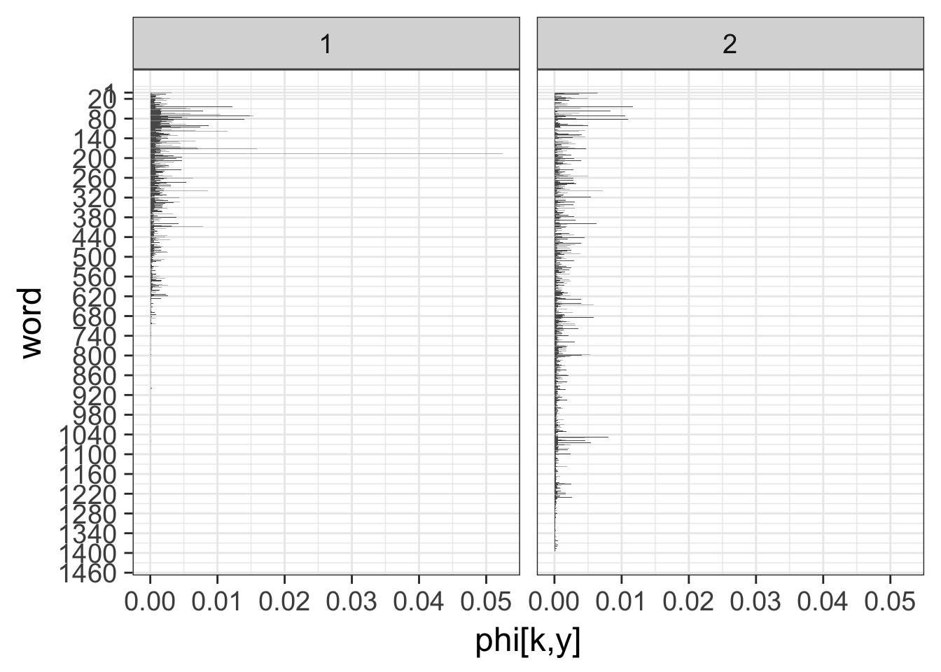
今後は各論文を横軸にとって、生起確率(MAP推定値)を縦軸にプロットしています。こうみると、二つのトピックそれぞれに違う論文が反応している様子がわかります。
ms <- rstan::extract(fit_vb)

probs <- c(0.1, 0.25, 0.5, 0.75, 0.9)
idx <- expand.grid(1:M, 1:K)
d_qua=NULL

d_qua <- t(apply(idx, 1, function(x) quantile(ms$theta[,x[1],x[2]],probs=probs)))
d_qua <- data.frame(idx, d_qua)

colnames(d_qua) <- c('article', 'topic', paste0('p', probs*100))

best.topic=NULL
for(i in 1:48){
aaa<-subset(d_qua,article==i)
best.topic<-c(best.topic,max.col(t(aaa$p50)))
}


p <- ggplot(d_qua, aes(x=article, y=p50,col=as.factor(topic)))
p <- p +geom_point()
p <- p + facet_wrap(~as.factor(topic))
p +theme_bw()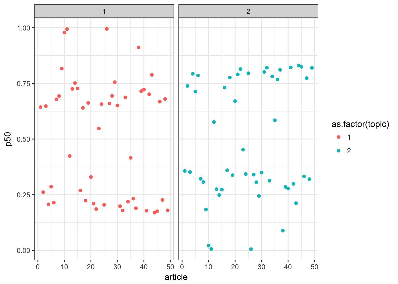
論文を該当する確率の高い方のトピックわりふって、docs.newからトピックグループごとのCorpusを抜き出します。そしてグループごとの頻出語を検討します。
A<-which(best.topic==1)
B<-which(best.topic==2)

dtm.A<-DocumentTermMatrix(docs.new[A])
dtm.B<-DocumentTermMatrix(docs.new[B])

freqA <- colSums(as.matrix(dtm.A))
ordA <- order(freqA,decreasing=TRUE)
freq20A<-data.frame(head(freqA[ordA],50))
freq20A$wordA<-rownames(freq20A)
names(freq20A)<-c("freq","word")

freqB <- colSums(as.matrix(dtm.B))
ordB <- order(freqB,decreasing=TRUE)
freq20B<-data.frame(head(freqB[ordB],50))
freq20B$wordB<-rownames(freq20B)
names(freq20B)<-c("freq","word")
freqs<-data.frame(freq20A$word,freq20B$word,rank=1:50)

kable(freqs)| freq20A.word | freq20B.word | rank |
|---|---|---|
| differ | effect | 1 |
| model | model | 2 |
| bayesian | studi | 3 |
| sampl | data | 4 |
| studi | patient | 5 |
| hiv | cancer | 6 |
| data | mirna | 7 |
| preval | diseas | 8 |
| risk | associ | 9 |
| rang | main | 10 |
| women | bayesian | 11 |
| analysi | event | 12 |
| water | colon | 13 |
| provinc | epistat | 14 |
| inform | dcl | 15 |
| imag | outcom | 16 |
| age | approach | 17 |
| decis | perform | 18 |
| class | comput | 19 |
| screen | stage | 20 |
| estim | inform | 21 |
| south | provid | 22 |
| treatment | estim | 23 |
| perform | structur | 24 |
| breast | indic | 25 |
| meta | random | 26 |
| spatial | treatment | 27 |
| classif | trial | 28 |
| control | analysi | 29 |
| popul | control | 30 |
| paramet | develop | 31 |
| effici | includ | 32 |
| compar | framework | 33 |
| describ | signific | 34 |
| account | target | 35 |
| heterogen | laparotomi | 36 |
| provinci | support | 37 |
| sexual | correl | 38 |
| survey | covari | 39 |
| outcom | identifi | 40 |
| cancer | question | 41 |
| percentag | base | 42 |
| prefer | process | 43 |
| genet | censor | 44 |
| present | featur | 45 |
| rate | observ | 46 |
| scale | phenotyp | 47 |
| time | anti | 48 |
| pcr | month | 49 |
| sourc | benefit | 50 |
あとは、グループごとにwordcloudを作成してやれば、本日の任務は完了です。上位の単語はあまり変わらないので見た目があまり変わらないので今回は面白くないですが、細かく見ていると、右の図の方が、infection、patient、response、 clinical、といった臨床関連用語が散見されるので医学的な研究のグループとしてまとめられているように思います (テキトー)。
library(wordcloud)
library(dplyr)
par(mfrow=c(1,2))
wordcloud::wordcloud(docs.new[A], scale = c(4.5, 0.4), max.words = 200,
          min.freq = 1, random.color=T, random.order = FALSE, rot.per = 0.00,
          use.r.layout = F, colors = brewer.pal(3, "Paired"),
          family="Helvetica")

wordcloud::wordcloud(docs.new[B], scale = c(4.5, 0.4), max.words = 200,
          min.freq = 5, random.color=T, random.order = FALSE, rot.per = 0.00,
          use.r.layout = F, colors = brewer.pal(3, "Paired"),
          family="Helvetica")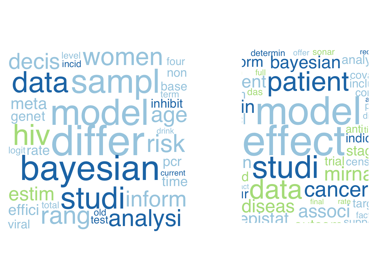
感想
stanでLDA、モデルはシンプルだけど、結構重たい処理になるので、高速化をどうするか。RでLDA用の便利な関数(topicmodelsなど)が続々と出てるので、それでまずはtopicmodelに親しむのはあり。gensimなど、HDPに挑戦していきたい。